http://en.wikipedia.org/wiki/Maximum_power_transfer_theorem


Maximum power transfer theorem
From Wikipedia, the free encyclopedia
In electrical engineering, the maximum power transfer theorem states that, to obtain maximum external power from a source with a finite internal resistance, the resistance of the load must equal the resistance of the source as viewed from its output terminals. Moritz von Jacobi published the maximum power (transfer) theorem around 1840; it is also referred to as "Jacobi's law".[1]
The theorem results in maximum power transfer, and not maximum efficiency. If the resistance of the load is made larger than the resistance of the source, then efficiency is higher, since a higher percentage of the source power is transferred to the load, but themagnitude of the load power is lower since the total circuit resistance goes up.
If the load resistance is smaller than the source resistance, then most of the power ends up being dissipated in the source, and although the total power dissipated is higher, due to a lower total resistance, it turns out that the amount dissipated in the load is reduced.
The theorem states how to choose (so as to maximize power transfer) the load resistance, once the source resistance is given. It is a common misconception to apply the theorem in the opposite scenario. It does not say how to choose the source resistance for a given load resistance. In fact, the source resistance that maximizes power transfer is always zero, regardless of the value of the load resistance.
The theorem can be extended to AC circuits that include reactance, and states that maximum power transfer occurs when the loadimpedance is equal to the complex conjugate of the source impedance.
Contents[hide] |
[edit]Maximizing power transfer versus power efficiency
The theorem was originally misunderstood (notably by Joule) to imply that a system consisting of an electric motor driven by a battery could not be more than 50% efficient since, when the impedances were matched, the power lost as heat in the battery would always be equal to the power delivered to the motor. In 1880 this assumption was shown to be false by either Edison or his colleague Francis Robbins Upton, who realized that maximum efficiency was not the same as maximum power transfer. To achieve maximum efficiency, the resistance of the source (whether a battery or a dynamo) could be made close to zero. Using this new understanding, they obtained an efficiency of about 90%, and proved that the electric motor was a practical alternative to the heat engine.


The condition of maximum power transfer does not result in maximum efficiency. If we define the efficiency  as the ratio of power dissipated by the load to power developed by the source, then it is straightforward to calculate from the above circuit diagram that
as the ratio of power dissipated by the load to power developed by the source, then it is straightforward to calculate from the above circuit diagram that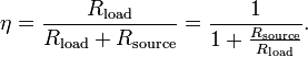
Consider three particular cases:
- If
 , then
- If
 or
or  then
then 
- If
 , then
The efficiency is only 50% when maximum power transfer is achieved, but approaches 100% as the load resistance approaches infinity, though the total power level tends towards zero. Efficiency also approaches 100% if the source resistance can be made close to zero. When the load resistance is zero, all the power is consumed inside the source (the power dissipated in a short circuit is zero) so the efficiency is zero.
[edit]Impedance matching
Main article: impedance matching
A related concept is reflectionless impedance matching. In radio, transmission lines, and other electronics, there is often a requirement to match the source impedance (such as a transmitter) to the load impedance (such as an antenna) to avoid reflections in the transmission line.
[edit]Calculus-based proof for purely resistive circuits
(See Cartwright[2] for a non-calculus-based proof)

In the diagram opposite, power is being transferred from the source, with voltage  and fixed source resistance
  , to a load with resistance
  , resulting in a current
  . By Ohm's law, is simply the source voltage divided by the total circuit resistance:
and fixed source resistance , to a load with resistance , resulting in a current . By Ohm's law, is simply the source voltage divided by the total circuit resistance:
The power  dissipated in the load is the square of the current multiplied by the resistance:
dissipated in the load is the square of the current multiplied by the resistance:
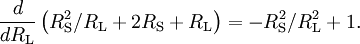
The value of for which this expression is a maximum could be calculated by differentiating it, but it is easier to calculate the value of for which the denominator
for which this expression is a maximum could be calculated by differentiating it, but it is easier to calculate the value of for which the denominator
is a minimum. The result will be the same in either case. Differentiating the denominator with respect to :
:
For a maximum or minimum, the first derivative is zero, so

or

In practical resistive circuits, and are both positive, so the positive sign in the above is the correct solution. To find out whether this solution is a minimum or a maximum, the denominator expression is differentiated again:
and are both positive, so the positive sign in the above is the correct solution. To find out whether this solution is a minimum or a maximum, the denominator expression is differentiated again:
This is always positive for positive values of and , showing that the denominator is a minimum, and the power is therefore a maximum, when
and , showing that the denominator is a minimum, and the power is therefore a maximum, when
A note of caution is in order here. This last statement, as written, implies to many people that for a given load, the source resistance must be set equal to the load resistance for maximum power transfer. However, this equation only applies if the source resistance cannot be adjusted, e.g., with antennas (see the first line in the proof stating "fixed source resistance"). For any given load resistance a source resistance of zero is the way to transfer maximum power to the load. As an example, a 100 volt source with an internal resistance of 10 ohms connected to a 10 ohm load will deliver 250 watts to that load. Make the source resistance zero ohms and the load power jumps to 1000 watts.
[edit]In reactive circuits
The theorem also applies where the source and/or load are not totally resistive. This invokes a refinement of the maximum power theorem, which says that any reactive components of source and load should be of equal magnitude but opposite phase. (See below for a derivation.) This means that the source and load impedances should be complex conjugates of each other. In the case of purely resistive circuits, the two concepts are identical. However, physically realizable sources and loads are not usually totally resistive, having some inductive or capacitive components, and so practical applications of this theorem, under the name of complex conjugate impedance matching, do, in fact, exist.
If the source is totally inductive (capacitive), then a totally capacitive (inductive) load, in the absence of resistive losses, would receive 100% of the energy from the source but send it back after a quarter cycle. The resultant circuit is nothing other than a resonant LC circuit in which the energy continues to oscillate to and fro. This is called reactive power. Power factor correction(where an inductive reactance is used to "balance out" a capacitive one), is essentially the same idea as complex conjugate impedance matching although it is done for entirely different reasons.
For a fixed reactive source, the maximum power theorem maximizes the real power (P) delivered to the load by complex conjugate matching the load to the source.
For a fixed reactive load, power factor correction minimizes the apparent power (S) (and unnecessary current) conducted by the transmission lines, while maintaining the same amount of real power transfer. This is done by adding a reactance to the load to balance out the load's own reactance, changing the reactive load impedance into a resistive load impedance.
[edit]Proof

In this diagram, AC power is being transferred from the source, with phasor magnitude voltage  (peak voltage) and fixed source impedance
  , to a load with impedance
  , resulting in a phasor magnitude current
  . is simply the source voltage divided by the total circuit impedance:
(peak voltage) and fixed source impedance , to a load with impedance , resulting in a phasor magnitude current . is simply the source voltage divided by the total circuit impedance: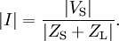
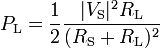
The average power  dissipated in the load is the square of the current multiplied by the resistive portion (the real part)
  of the load impedance:
dissipated in the load is the square of the current multiplied by the resistive portion (the real part) of the load impedance:
where the resistance  and reactance
  are the real and imaginary parts of , and
  is the imaginary part of .
and reactance are the real and imaginary parts of , and is the imaginary part of .
To determine the values of and (since  , , and are fixed) for which this expression is a maximum, we first find, for each fixed positive value of , the value of the reactive term for which the denominator
and (since , , and are fixed) for which this expression is a maximum, we first find, for each fixed positive value of , the value of the reactive term for which the denominator
is a minimum. Since reactances can be negative, this denominator is easily minimized by making

The power equation is now reduced to:
and it remains to find the value of which maximizes this expression. However, this maximization problem has exactly the same form as in the purely resistive case, and the maximizing condition  can be found in the same way.
which maximizes this expression. However, this maximization problem has exactly the same form as in the purely resistive case, and the maximizing condition can be found in the same way.
The combination of conditions


can be concisely written with a complex conjugate (the *) as:

- http://www.tina.com/English/tina/course/11maxim/maxim
MAXIMUM POWER TRANSFER THEOREM
- Definition
- Sometimes in engineering we are asked to design a circuit that will transfer the maximum power to a load from a given source. According to the maximum power transfer theorem, a load will receive maximum power from a source when its resistance (RL) is equal to the internal resistance (RI) of the source. If the source circuit is already in the form of a Thevenin or Norton equivalent circuit (a voltage or current source with an internal resistance), then the solution is simple. If the circuit is not in the form of a Thevenin or Norton equivalent circuit, we must first use Thevenin’s orNorton’s theorem to obtain the equivalent circuit.Here’s how to arrange for the maximum power transfer.1. Find the internal resistance, RI. This is the resistance one finds by looking back into the two load terminals of the source with no load connected. As we have shown in the Thevenin’s Theorem and Norton’s Theorem chapters, the easiest method is to replace voltage sources by short circuits and current sources by open circuits, then find the total resistance between the two load terminals.2. Find the open circuit voltage (UT) or the short circuit current (IN) of the source between the two load terminals, with no load connected.Once we have found RI, we know the optimal load resistance
(RLopt = RI). Finally, the maximum power can be found In addition to the maximum power, we might want to know another important quantity: the efficiency. Efficiency is defined by the ratio of the power received by the load to the total power supplied by the source. For the Thevenin equivalent:
and for the Norton equivalent:Using TINA’s Interpreter, it is easy to draw P, P/Pmax, and h as a function of RL. The next graph shows P/Pmax, the power on RL divided by the maximum power, Pmax, as a function of RL (for a circuit with internal resistance RI=50).
Now let’s see the efficiency h as a function of RL. The circuit and the TINA Interpreter program to draw the diagrams above are shown below. Note that we we also used the editing tools of TINA’s Diagram window to add some text and the dotted line.
 Now let’s explore the efficiency (h) for the case of maximum power transfer, where RL = RTh.The efficiency is:
 which when given as a percentage is only 50%. This is acceptable for some applications in electronics and telecommunication, such as amplifiers, radio receivers or transmitters However, 50% efficiency is not acceptable for batteries, power supplies, and certainly not for power plants.Another undesirable consequence of arranging a load to achieve maximum power transfer is the 50% voltage drop on the internal resistance. A 50% drop in source voltage can be a real problem. What is needed, in fact, is a nearly constant load voltage. This calls for systems where the internal resistance of the source is much lower than the load resistance. Imagine a 10 GW power plant operating at or close to maximum power transfer. This would mean that half of the energy generated by the plant would be dissipated in the transmission lines and in the generators (which would probably burn out). It would also result in load voltages that would randomly fluctuate between 100% and 200% of the nominal value as consumer power usage varied.To illustrate the application of the maximum power transfer theorem, let’s find the optimum value of the resistor RL to receive maximum power in the circuit below.
Click/tap the circuit above to analyze on-line or click this link to Save under Windows We get the maximum power if RL= R1, so RL = 1 kohm. The maximum power: A similar problem, but with a current source:
Click/tap the circuit above to analyze on-line or click this link to Save under Windows Find the maximum power of the resistor RL .We get the maximum power if RL = R1 = 8 ohm. The maximum power: The following problem is more complex, so first we must reduce it to a simpler circuit.Find RI to achieve maximum power transfer, and calculate this maximum power.
Click/tap the circuit above to analyze on-line or click this link to Save under Windows
First find the Norton equivalent using TINA.
Click/tap the circuit above to analyze on-line or click this link to Save under Windows Finally the maximum power:
 {Solution by TINA's Interpreter}
O1:=Replus(R4,(R1+Replus(R2,R3)))/(R+Replus(R4,(R1+Replus(R2,R3))));
IN:=Vs*O1*Replus(R2,R3)/(R1+Replus(R2,R3))/R3;
RN:=R3+Replus(R2,(R1+Replus(R,R4)));
Pmax:=sqr(IN)/4*RN;
IN=[250u]
RN=[80k]
Pmax=[1.25m]We can also solve this problem using one of TINA’s most interesting features, the Optimization analysis mode.To set up for an Optimization, use the Analysis menu or the icons at the top right of the screen and select Optimization Target. Click on the Power meter to open its dialog box and select Maximum. Next, select Control Object, click on RI, and set the limits within which the optimum value should be searched.To carry out the optimization in TINA v6 and above, simply use the Analysis/Optimization/DC Optimization command from the Analysis menu.In older versions of TINA, you can set this mode from the menu, Analysis/Mode/Optimization, and then execute a DC Analysis.After running Optimization for the problem above, the following screen appears: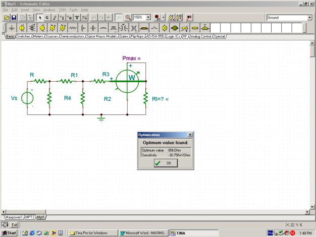 After Optimization, the value of RI is automatically updated to the value found. If we next run an interactive DC analysis by pressing the DC button, the maximum power is displayed as shown in the following figure.
No comments:
Post a Comment