http://en.wikipedia.org/wiki/Elliptic_filter
Elliptic filter
An elliptic filter (also known as a Cauer filter, named after Wilhelm Cauer) is asignal processing filter with equalized ripple (equiripple) behavior in both the passbandand the stopband. The amount of ripple in each band is independently adjustable, and no other filter of equal order can have a faster transition in gain between the passbandand the stopband, for the given values of ripple (whether the ripple is equalized or not). Alternatively, one may give up the ability to independently adjust the passband and stopband ripple, and instead design a filter which is maximally insensitive to component variations.
As the ripple in the stopband approaches zero, the filter becomes a type I Chebyshev filter. As the ripple in the passband approaches zero, the filter becomes a type IIChebyshev filter and finally, as both ripple values approach zero, the filter becomes aButterworth filter.
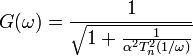
The gain of a lowpass elliptic filter as a function of angular frequency ω is given by:

where Rn is the nth-order elliptic rational function (sometimes known as a Chebyshev rational function) and
 is the cutoff frequency
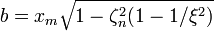
 is the ripple factor
 is the selectivity factor
The value of the ripple factor specifies the passband ripple, while the combination of the ripple factor and the selectivity factor specify the stopband ripple.
Contents[hide] |
[edit]Properties
.svg)
.svg)
- In the passband, the elliptic rational function varies between zero and unity. The passband of the gain therefore will vary between 1 and
 .
.
- In the stopband, the elliptic rational function varies between infinity and the discrimination factor
 which is defined as:

- The gain of the stopband therefore will vary between 0 and
 .
.
- In the limit of
 the elliptic rational function becomes a Chebyshev polynomial, and therefore the filter becomes a Chebyshev type I filter, with ripple factor ε
- Since the Butterworth filter is a limiting form of the Chebyshev filter, it follows that in the limit of ,
 and
and  such that
  the filter becomes aButterworth filter
- In the limit of , and such that
 and
and  , the filter becomes aChebyshev type II filter with gain
[edit]Poles and zeroes
.svg)
 . The white spots are poles and the black spots are zeroes. There are a total of 16 poles and 8 double zeroes. What appears to be a single pole and zero near the transition region is actually four poles and two double zeroes as shown in the expanded view below. In this image, black corresponds to a gain of 0.0001 or less and white corresponds to a gain of 10 or more.
.svg)
The zeroes of the gain of an elliptic filter will coincide with the poles of the elliptic rational function, which are derived in the article on elliptic rational functions.
The poles of the gain of an elliptic filter may be derived in a manner very similar to the derivation of the poles of the gain of a type I Chebyshev filter. For simplicity, assume that the cutoff frequency is equal to unity. The poles  of the gain of the elliptical filter will be the zeroes of the denominator of the gain. Using the complex frequency
  this means that:
of the gain of the elliptical filter will be the zeroes of the denominator of the gain. Using the complex frequency this means that:
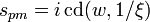
Defining  where cd() is the Jacobi elliptic cosine function and using the definition of the elliptic rational functions yields:
where cd() is the Jacobi elliptic cosine function and using the definition of the elliptic rational functions yields: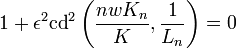
where 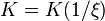 and
and  . Solving for w
and . Solving for w
where the multiple values of the inverse cd() function are made explicit using the integer index m.
The poles of the elliptic gain function are then:
As is the case for the Chebyshev polynomials, this may be expressed in explicitly complex form (Lutovac & et al. 2001, § 12.8)


where  is a function of
  and and
  are the zeroes of the elliptic rational function. is expressible for all n in terms of Jacobi elliptic functions, or algebraically for some orders, especially orders 1,2, and 3. For orders 1 and 2 we have
is a function of and and are the zeroes of the elliptic rational function. is expressible for all n in terms of Jacobi elliptic functions, or algebraically for some orders, especially orders 1,2, and 3. For orders 1 and 2 we have
where
The algebraic expression for  is rather involved (See Lutovac & et al. (2001, § 12.8.1)).
is rather involved (See Lutovac & et al. (2001, § 12.8.1)).
The nesting property of the elliptic rational functions can be used to build up higher order expressions for :
:
where  .
.
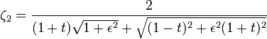
.[edit]Minimum Q-factor elliptic filters

See Lutovac & et al. (2001, § 12.11, 13.14).
Elliptic filters are generally specified by requiring a particular value for the passband ripple, stopband ripple and the sharpness of the cutoff. This will generally specify a minimum value of the filter order which must be used. Another design consideration is the sensitivity of the gain function to the values of the electronic components used to build the filter. This sensitivity is inversely proportional to the quality factor (Q-factor) of the poles of the transfer function of the filter. The Q-factor of a pole is defined as:
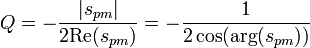
and is a measure of the influence of the pole on the gain function. For an elliptic filter, it happens that, for a given order, there exists a relationship between the ripple factor and selectivity factor which simultaneously minimizes the Q-factor of all poles in the transfer function:

This results in a filter which is maximally insensitive to component variations, but the ability to independently specify the passband and stopband ripples will be lost. For such filters, as the order increases, the ripple in both bands will decrease and the rate of cutoff will increase. If one decides to use a minimum-Q elliptic filter in order to achieve a particular minimum ripple in the filter bands along with a particular rate of cutoff, the order needed will generally be greater than the order one would otherwise need without the minimum-Q restriction. An image of the absolute value of the gain will look very much like the image in the previous section, except that the poles are arranged in a circle rather than an ellipse. They will not be evenly spaced and there will be zeroes on the ω axis, unlike the Butterworth filter, whose poles are also arranged in a circle.
[edit]Comparison with other linear filters
Here is an image showing the elliptic filter next to other common kind of filters obtained with the same number of coefficients:

As is clear from the image, elliptic filters are sharper than all the others, but they show ripples on the whole bandwidth.
No comments:
Post a Comment